Julia on Titanic

This is an introduction to Data Analysis and Decision Trees using Julia. In this tutorial we will explore how to tackle Kaggle’s Titanic competition using Julia and Machine Learning. This tutorial is adopted from the Kaggle R tutorial on Machine Learning on Datacamp In case you’re new to Julia, you can read more about its awesomeness on julialang.org.
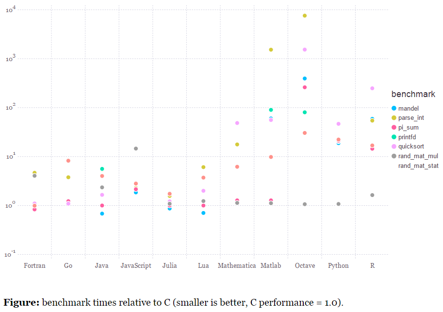
Again, the point of this tutorial is not to teach machine learning but to provide a starting point to get your hands dirty with Julia code. The benchmark numbers on the Julia website look pretty impressive. So get ready to embrace Julia with a warm hug!

Let’s get started. We will mostly be using 3 main packages from Julia ecosystem

• DataFrames
• Gadfly
• DecisionTree

We start with loading the dataset from the Titanic Competition from kaggle. We will use readtable for that and inspect the first few data points with head() on the loaded DataFrame. We will use the already split train and test sets from DataCamp training set: http://s3.amazonaws.com/assets.datacamp.com/course/Kaggle/train.csv test set: http://s3.amazonaws.com/assets.datacamp.com/course/Kaggle/test.csv I have them downloaded in the data directory.

using DataFrames


train = readtable("data/train.csv")
head(train)

	PassengerId	Survived	Pclass	Name	Sex	Age	SibSp	Parch	Ticket	Fare	Cabin	Embarked
1	1	0	3	Braund, Mr. Owen Harris	male	22.0	1	0	A/5 21171	7.25	NA	S
2	2	1	1	Cumings, Mrs. John Bradley (Florence Briggs Thayer)	female	38.0	1	0	PC 17599	71.2833	C85	C
3	3	1	3	Heikkinen, Miss. Laina	female	26.0	0	0	STON/O2. 3101282	7.925	NA	S
4	4	1	1	Futrelle, Mrs. Jacques Heath (Lily May Peel)	female	35.0	1	0	113803	53.1	C123	S
5	5	0	3	Allen, Mr. William Henry	male	35.0	0	0	373450	8.05	NA	S
6	6	0	3	Moran, Mr. James	male	NA	0	0	330877	8.4583	NA	Q

test = readtable("data/test.csv")
head(test)

	PassengerId	Pclass	Name	Sex	Age	SibSp	Parch	Ticket	Fare	Cabin	Embarked
1	892	3	Kelly, Mr. James	male	34.5	0	0	330911	7.8292	NA	Q
2	893	3	Wilkes, Mrs. James (Ellen Needs)	female	47.0	1	0	363272	7.0	NA	S
3	894	2	Myles, Mr. Thomas Francis	male	62.0	0	0	240276	9.6875	NA	Q
4	895	3	Wirz, Mr. Albert	male	27.0	0	0	315154	8.6625	NA	S
5	896	3	Hirvonen, Mrs. Alexander (Helga E Lindqvist)	female	22.0	1	1	3101298	12.2875	NA	S
6	897	3	Svensson, Mr. Johan Cervin	male	14.0	0	0	7538	9.225	NA	S

size(train, 1)




891

Let’s take a closer look at our datasets. describe() helps us to summarize the entire dataset.

describe(train)

PassengerId
Min      1.0
1st Qu.  223.5
Median   446.0
Mean     446.0
3rd Qu.  668.5
Max      891.0
NAs      0
NA%      0.0%

Survived
Min      0.0
1st Qu.  0.0
Median   0.0
Mean     0.3838383838383838
3rd Qu.  1.0
Max      1.0
NAs      0
NA%      0.0%

Pclass
Min      1.0
1st Qu.  2.0
Median   3.0
Mean     2.308641975308642
3rd Qu.  3.0
Max      3.0
NAs      0
NA%      0.0%

Name
Length  891
Type    UTF8String
NAs     0
NA%     0.0%
Unique  891

Sex
Length  891
Type    UTF8String
NAs     0
NA%     0.0%
Unique  2

Age
Min      0.42
1st Qu.  20.125
Median   28.0
Mean     29.69911764705882
3rd Qu.  38.0
Max      80.0
NAs      177
NA%      19.87%

SibSp
Min      0.0
1st Qu.  0.0
Median   0.0
Mean     0.5230078563411896
3rd Qu.  1.0
Max      8.0
NAs      0
NA%      0.0%

Parch
Min      0.0
1st Qu.  0.0
Median   0.0
Mean     0.38159371492704824
3rd Qu.  0.0
Max      6.0
NAs      0
NA%      0.0%

Ticket
Length  891
Type    UTF8String
NAs     0
NA%     0.0%
Unique  681

Fare
Min      0.0
1st Qu.  7.9104
Median   14.4542
Mean     32.20420796857464
3rd Qu.  31.0
Max      512.3292
NAs      0
NA%      0.0%

Cabin
Length  891
Type    UTF8String
NAs     687
NA%     77.1%
Unique  148

Embarked
Length  891
Type    UTF8String
NAs     2
NA%     0.22%
Unique  4

If you want to just check the datatypes of the columns you can use eltypes()

eltypes(train)




12-element Array{Type{T<:Top},1}:
 Int64     
 Int64     
 Int64     
 UTF8String
 UTF8String
 Float64   
 Int64     
 Int64     
 UTF8String
 Float64   
 UTF8String
 UTF8String

Data Analysis

Let’s get our hand real dirty now. We want to check how many people survived the disaster. Its good to know how the distribution looks like on the classification classes.

counts() will give you a frequency table, but it does not tell you how the split is. It is the equivalent of table() in R.

counts(train[:Survived])




2-element Array{Int64,1}:
 549
 342

countmap() for rescue! Countmap gives you a dictionary of value => frequency

countmap(train[:Survived])




Dict{Union(NAtype,Int64),Int64} with 2 entries:
  0 => 549
  1 => 342

If you want proportions like prop.table() in R, you can use proportions() or proportionmap()

proportions(train[:Survived])




2-element Array{Float64,1}:
 0.616162
 0.383838




proportionmap(train[:Survived])




Dict{Union(NAtype,Int64),Float64} with 2 entries:
  0 => 0.6161616161616161
  1 => 0.3838383838383838

Counts does not work for categorical variables, so you can use countmap() there.

countmap(train[:Sex])

Dict{Union(NAtype,UTF8String),Int64} with 2 entries:
  "male"   => 577
  "female" => 314

Now that we know the split between male and female population on Titanic and the proportions that survived, let check if the sex of a person had an impact on the chances of surviving.
We will examine this using a stacked histogram of Sex vs Survived using Gadfly package.

using Gadfly


plot(train, x="Sex", y="Survived", color="Survived", Geom.histogram(position=:stack), Scale.color_discrete_manual("red","green"))

Its pretty clear that more females survived over males.
So let’s predict Survived=1 if Sex=female else Survived=0. With that you have your first predictive model ready!!

But let’s not stop there, we have lot more dimensions to the data. Let’s see if we can make use of those to enhance the model. We have Age as one of the columns, using which we can create another dimension to the data - a variable indicating whether the person was a child or not.

train[:Child] = 1
train[isna(train[:Age]), :Child] = 1 #this can be avoided. Its just an explicit way to demonstrate the rule
train[train[:Age] .< 18, :Child] = 1 #same applies for this, as all Child fields are 1 by default except when Age >= 18
train[train[:Age] .>= 18, :Child] = 0
head(train)

	PassengerId	Survived	Pclass	Name	Sex	Age	SibSp	Parch	Ticket	Fare	Cabin	Embarked	Child
1	1	0	3	Braund, Mr. Owen Harris	male	22.0	1	0	A/5 21171	7.25	NA	S	0
2	2	1	1	Cumings, Mrs. John Bradley (Florence Briggs Thayer)	female	38.0	1	0	PC 17599	71.2833	C85	C	0
3	3	1	3	Heikkinen, Miss. Laina	female	26.0	0	0	STON/O2. 3101282	7.925	NA	S	0
4	4	1	1	Futrelle, Mrs. Jacques Heath (Lily May Peel)	female	35.0	1	0	113803	53.1	C123	S	0
5	5	0	3	Allen, Mr. William Henry	male	35.0	0	0	373450	8.05	NA	S	0
6	6	0	3	Moran, Mr. James	male	NA	0	0	330877	8.4583	NA	Q	1

Now that we have our Child indicator variable, let’s try to plot the survival rate of children on Titanic.

plot(train, x="Child", y="Survived", color="Survived", Geom.histogram(position=:stack), Scale.color_discrete_manual("red","green"))

We see the number of Children survived is lower than the number of victims.

Let try to combine the gender and child variables to see how that impacts the survival rate. We go back to our friendly bug Gadfly to construct a stacked histogram with subplots.

plot(train, xgroup="Child", x="Sex", y="Survived", color="Survived", Geom.subplot_grid(Geom.histogram(position=:stack)), Scale.color_discrete_manual("red","green"))

These kind of visual analysis is a powerful tool to perform the initial data mining before diving into any deeper machine learning algorithms for predictions.

We clearly see that Age and Gender influence the survival. But we cannot generate all combinations to create a ifelse model for prediction. Enter DecisionTrees. Decision trees do exactly what we did with Gender but at a larger scale where all dimensions (or features) are invovled in forming the decision tree.
In our case the decision we need to make is Survived or Not.

Before doing that we need to handle the missing data in our feature variables. There are multiple ways to handle missing data and we wont go deeper into them. We will use a simple technique of filling the missing value with

1. Mean value if the variable is numeric.
2. Max frequency categorical variable value for categorical variables.

From describe() above we have seen that Embarked and Age have some missing values (NA)

countmap(train[:Embarked])

Dict{Union(NAtype,UTF8String),Int64} with 4 entries:
  "Q" => 77
  "S" => 644
  "C" => 168
  NA  => 2

train[isna(train[:Embarked]), :Embarked] = "S"

"S"

meanAge = mean(train[!isna(train[:Age]), :Age])

29.69911764705882

train[isna(train[:Age]), :Age] = meanAge

29.69911764705882

Now that we knocked out the NAs out of our way, let’s roll up our sleeves and grow a decision tree! We will be using the DecisionTree julia package.
Features form the predictors and labels are the response variables for the decision tree. We will start with building the Arrays for features and labels.

using DecisionTree

train[:Age] = float64(train[:Age])
train[:Fare] = float64(train[:Fare])
features = array(train[:,[:Pclass, :Sex, :Age, :SibSp, :Parch, :Fare, :Embarked, :Child]])
labels=array(train[:Survived])


891-element Array{Int64,1}:
 0
 1
 1
 1
 0
 0
 0
 0
 1
 1
 1
 1
 0
 ⋮
 1
 1
 0
 0
 0
 0
 0
 0
 1
 0
 1
 0


features

891x8 Array{Any,2}:
 3  "male"    22.0     1  0   7.25    "S"  0
 1  "female"  38.0     1  0  71.2833  "C"  0
 3  "female"  26.0     0  0   7.925   "S"  0
 1  "female"  35.0     1  0  53.1     "S"  0
 3  "male"    35.0     0  0   8.05    "S"  0
 3  "male"    29.6991  0  0   8.4583  "Q"  1
 1  "male"    54.0     0  0  51.8625  "S"  0
 3  "male"     2.0     3  1  21.075   "S"  1
 3  "female"  27.0     0  2  11.1333  "S"  0
 2  "female"  14.0     1  0  30.0708  "C"  1
 3  "female"   4.0     1  1  16.7     "S"  1
 1  "female"  58.0     0  0  26.55    "S"  0
 3  "male"    20.0     0  0   8.05    "S"  0
 ⋮                            ⋮             
 1  "female"  56.0     0  1  83.1583  "C"  0
 2  "female"  25.0     0  1  26.0     "S"  0
 3  "male"    33.0     0  0   7.8958  "S"  0
 3  "female"  22.0     0  0  10.5167  "S"  0
 2  "male"    28.0     0  0  10.5     "S"  0
 3  "male"    25.0     0  0   7.05    "S"  0
 3  "female"  39.0     0  5  29.125   "Q"  0
 2  "male"    27.0     0  0  13.0     "S"  0
 1  "female"  19.0     0  0  30.0     "S"  0
 3  "female"  29.6991  1  2  23.45    "S"  1
 1  "male"    26.0     0  0  30.0     "C"  0
 3  "male"    32.0     0  0   7.75    "Q"  0

Stumps

A stump is the simplest decision tree, with only one split and two classification nodes (leaves). It tries to generate a single split with most predictive power. This is performed by splitting the dataset into 2 subset and returning the split with highest information gain. We will use the build_stumps api from DecisionTree and feed it with the above generated labels and features.

stump = build_stump(labels, features)
print_tree(stump)

Feature 2, Threshold male
L-> 1 : 233/314
R-> 0 : 468/577

The stump picks feature 2, Sex to make the split with threshold being “male”. The interpretation being - all males data points to the right leaf and all female datapoints go to the left leaf. Hence the 314 on L and 577 on R - number of female and male datapoints (respectively) in train set.
L -> 1 implies Survived=1 is on left branch
R -> 0 implies Survived=0 is on right branch
This creates a basic 1-rules tree with deciding factor being gender of the person.

Let’s verify the split by predicting on the training data.

predictions = apply_tree(stump, features)
confusion_matrix(labels, predictions)

2x2 Array{Int64,2}:
 468   81
 109  233

Classes:  {0,1}
Matrix:   
Accuracy: 0.7867564534231201
Kappa:    0.5421129503407983

Since we predict male who survived and females who didnt survive wrongly we get a miclassification count of 81 + 109. This gives use an accuracy of 1-190/891 = 0.7867

Decision Trees

Now that we have our 1-level decision stump, lets bring it all together and build our first multi-split decision tree. We can use build_tree() which recursively splits the dataset till we get pure leaves which contain samples of only 1 class.

model = build_tree(labels, features)
print_tree(model, 5)
length(model)

Feature 2, Threshold male
L-> Feature 1, Threshold 3
    L-> Feature 6, Threshold 29.0
        L-> Feature 6, Threshold 28.7125
            L-> Feature 3, Threshold 24.0
                L-> 1 : 15/15
                R-> 
            R-> 0 : 1/1
        R-> Feature 3, Threshold 3.0
            L-> 0 : 1/1
            R-> Feature 5, Threshold 2
                L-> 1 : 84/84
                R-> 
    R-> Feature 6, Threshold 23.45
        L-> Feature 8, Threshold 1
            L-> Feature 3, Threshold 37.0
                L-> 
                R-> 
            R-> Feature 6, Threshold 15.5
                L-> 
                R-> 
        R-> Feature 5, Threshold 1
            L-> 1 : 1/1
            R-> Feature 6, Threshold 31.3875
                L-> 0 : 15/15
                R-> 
R-> Feature 6, Threshold 26.2875
    L-> Feature 3, Threshold 15.0
        L-> Feature 4, Threshold 3
            L-> Feature 3, Threshold 11.0
                L-> 1 : 12/12
                R-> 
            R-> 0 : 1/1
        R-> Feature 7, Threshold Q
            L-> Feature 6, Threshold 15.2458
                L-> 
                R-> 
            R-> Feature 6, Threshold 13.5
                L-> 
                R-> 
    R-> Feature 4, Threshold 3
        L-> Feature 3, Threshold 16.0
            L-> 1 : 7/7
            R-> Feature 6, Threshold 26.55
                L-> 1 : 4/4
                R-> 
        R-> Feature 3, Threshold 4.0
            L-> Feature 3, Threshold 3.0
                L-> 0 : 4/4
                R-> 1 : 1/1
            R-> 0 : 18/18





200

We get a large tree so we use the depth parameter of print_tree() to pretty print to a depth of 5.
We can count the number of leaves of our tree using length() on the tree model. Length of our tree is 200.

Although we have a nice looking decision tree ready, we have a bunch of problems - * our classifier is complex because of the tree size * our model overfits on the training data in an attempt to improve accuracy on each bucket. Notice

Solution - Tree Pruning

From wikipedia/Pruning_decision_tree

“Pruning is a technique in machine learning that reduces the size of decision trees by removing sections of the tree that provide little power to classify instances. Pruning reduces the complexity of the final classifier, and hence improves predictive accuracy by the reduction of overfitting.”

# prune tree: merge leaves having >= 70% combined purity (default: 100%)
model = prune_tree(model, 0.7)
# pretty print of the tree, to a depth of 5 nodes (optional)
print_tree(model, 5)
length(model)

Feature 2, Threshold male
L-> Feature 1, Threshold 3
    L-> Feature 6, Threshold 29.0
        L-> Feature 6, Threshold 28.7125
            L-> Feature 3, Threshold 24.0
                L-> 1 : 15/15
                R-> 
            R-> 0 : 1/1
        R-> 1 : 98/100
    R-> Feature 6, Threshold 23.45
        L-> Feature 8, Threshold 1
            L-> Feature 3, Threshold 37.0
                L-> 
                R-> 0 : 6/7
            R-> Feature 6, Threshold 15.5
                L-> 
                R-> 1 : 14/16
        R-> 0 : 24/27
R-> Feature 6, Threshold 26.2875
    L-> Feature 3, Threshold 15.0
        L-> Feature 4, Threshold 3
            L-> Feature 3, Threshold 11.0
                L-> 1 : 12/12
                R-> 
            R-> 0 : 1/1
        R-> Feature 7, Threshold Q
            L-> Feature 6, Threshold 15.2458
                L-> 
                R-> 1 : 4/6
            R-> Feature 6, Threshold 13.5
                L-> 
                R-> 0 : 62/64
    R-> Feature 4, Threshold 3
        L-> Feature 3, Threshold 16.0
            L-> 1 : 7/7
            R-> Feature 6, Threshold 26.55
                L-> 1 : 4/4
                R-> 
        R-> 0 : 22/23





125

Pruning is a bottom-up process which merges leaves into one leaf in a repeated fashion.
The merge criteria is based on the pruning parameter (0.7 in the example above). The pruning parameter is a purity threshold. If the combined purity of two adjacent leaves is greater than the pruning threshold then the two leaves are merged into one.

Length of our pruned tree is reduced to 125 from 200.

We can further reduce the number of leaves by reducing the threshold. But how do you know what is a good threshold ?
There are multiple techniques to determine that one of them being grid search where you try multiple thresholds, plot the number of trees with the threshold values to compare against each other.
One way to do this is using n-fold cross validation.
tl;dr - Cross validation breaks the dataset into train and test sets for measuring accuracy. N-fold CV does this by randomly partitioning the train set into N equal subsets and each subset is used once as a test set while others are used as train sets. Using this we get N prediction performance numbers.

# run n-fold cross validation for pruned tree,
purities = linspace(0.1, 1.0, 5)
accuracies = zeros(length(purities))

for i in 1:length(purities)
    accuracies[i] = mean(nfoldCV_tree(labels, features, purities[i], 5))
end

plot(x=purities, y=accuracies, Geom.point, Geom.line, Guide.xlabel("Threshold"), Guide.ylabel("Accuracy"), Guide.title("Pruning Comparison"))


Fold 1


2x2 Array{Int64,2}:
 111  0
  67  0



2x2 Array{Int64,2}:
 118  0
  60  0



Classes:  {0,1}
Matrix:   
Accuracy: 0.6235955056179775
Kappa:    0.0

Fold 2
Classes:  {0,1}
Matrix:   
Accuracy: 0.6629213483146067
Kappa:    0.0

Fold 


2x2 Array{Int64,2}:
 107  0
  71  0


3
Classes:  {0,1}
Matrix:   
Accuracy: 0.601123595505618
Kappa:    0.0

Fold 


2x2 Array{Int64,2}:
 111  0
  67  0



2x2 Array{Int64,2}:
 101  0
  77  0


4
Classes:  {0,1}
Matrix:   
Accuracy: 0.6235955056179775
Kappa:    0.0

Fold 5
Classes:  {0,1}
Matrix:   
Accuracy: 0.5674157303370787
Kappa:    0.0

Mean Accuracy: 0.6157303370786517

Fold 


2x2 Array{Int64,2}:
 110  0
  68  0



2x2 Array{Int64,2}:
 111  0
  67  0


1
Classes:  {0,1}
Matrix:   
Accuracy: 0.6179775280898876
Kappa:    0.0

Fold 2
Classes:  {0,1}
Matrix:   
Accuracy: 0.6235955056179775
Kappa:    0.0

Fold 


2x2 Array{Int64,2}:
 114  0
  64  0



2x2 Array{Int64,2}:
 107  0
  71  0


3
Classes:  {0,1}
Matrix:   
Accuracy: 0.6404494382022472
Kappa:    0.0

Fold 4
Classes:  {0,1}
Matrix:   
Accuracy: 0.601123595505618
Kappa:    0.0

Fold 


2x2 Array{Int64,2}:
 107  0
  71  0



2x2 Array{Int64,2}:
 87  20
 14  57


5
Classes:  {0,1}
Matrix:   
Accuracy: 0.601123595505618
Kappa:    0.0

Mean Accuracy: 0.6168539325842697

Fold 1
Classes:  {0,1}
Matrix:   
Accuracy: 0.8089887640449438
Kappa:    0.6072680077871512

Fold 


2x2 Array{Int64,2}:
 88  21
 22  47


2
Classes:  {0,1}
Matrix:   
Accuracy: 0.7584269662921348
Kappa:    0.4898013598186908

Fold 


2x2 Array{Int64,2}:
 98  16
 21  43



2x2 Array{Int64,2}:
 93  15
 23  47


3
Classes:  {0,1}
Matrix:   
Accuracy: 0.7921348314606742
Kappa:    0.5407892901966255

Fold 4
Classes:  {0,1}
Matrix:   
Accuracy: 0.7865168539325843
Kappa:    0.5434665226781858

Fold 


2x2 Array{Int64,2}:
 91  20
 17  50



2x2 Array{Int64,2}:
 95  17
 30  36


5
Classes:  {0,1}
Matrix:   
Accuracy: 0.7921348314606742
Kappa:    0.5611088897774225

Mean Accuracy: 0.7876404494382022

Fold 1
Classes:  {0,1}
Matrix:   
Accuracy: 0.7359550561797753
Kappa:    0.4102636402086564

Fold 


2x2 Array{Int64,2}:
 87  14
 28  49


2
Classes:  {0,1}
Matrix:   
Accuracy: 0.7640449438202247
Kappa:    0.5087396504139834

Fold 


2x2 Array{Int64,2}:
 80  23
 15  60



2x2 Array{Int64,2}:
 105  16
  10  47


3
Classes:  {0,1}
Matrix:   
Accuracy: 0.7865168539325843
Kappa:    0.5684573178512186

Fold 4
Classes:  {0,1}
Matrix:   
Accuracy: 0.8539325842696629
Kappa:    0.6735787840315982

Fold 


2x2 Array{Int64,2}:
 80  31
 16  51



2x2 Array{Int64,2}:
 95  23
 17  43


5
Classes:  {0,1}
Matrix:   
Accuracy: 0.7359550561797753
Kappa:    0.461439423200721

Mean Accuracy: 0.7752808988764045

Fold 1
Classes:  {0,1}
Matrix:   
Accuracy: 0.7752808988764045
Kappa:    0.5092362834298318

Fold 


2x2 Array{Int64,2}:
 91  20
 21  46



2x2 Array{Int64,2}:
 99  11
 18  50


2
Classes:  {0,1}
Matrix:   
Accuracy: 0.7696629213483146
Kappa:    0.5078894133513149

Fold 3
Classes:  {0,1}
Matrix:   
Accuracy: 0.8370786516853933
Kappa:    0.6480294558843585

Fold 


2x2 Array{Int64,2}:
 87  19
 21  51



2x2 Array{Int64,2}:
 77  26
 26  49


4
Classes:  {0,1}
Matrix:   
Accuracy: 0.7752808988764045
Kappa:    0.5314556462226901

Fold 5
Classes:  {0,1}
Matrix:   
Accuracy: 0.7078651685393258
Kappa:    0.4009061488673138

Mean Accuracy: 0.7730337078651685

It seems we get the highest accuracy is at a threshold just above 0.5

Conclusion

We saw how easy it is to get your hands dirty in Julia waters. Decision trees are pretty effective but they are slower to train on large datasets, but once trained the predictions are fast - just a walk down the tree.

• ← Previous Post
• Next Post →

---